Snakes and Ladders: Simulation, Markov Chains, and Board Design
Lately, my son has been obsessed with the game of Snakes and Ladders. So much so that he made it a mission to win the game first before he does any thing else. Watching him play so many games, I got curious about the game mechanics and design. In this post I explored questions like - what is the expected number of turns in a game, what a boring Snakes and Ladders board with extremely low variance would look like, and conversely, how to mathematically design a chaotic board where the variance is very high.
Simulating a Game
Let’s start by simulating a single game with two players on the board that we got from the store.
Understanding Game Statistics via Monte Carlo
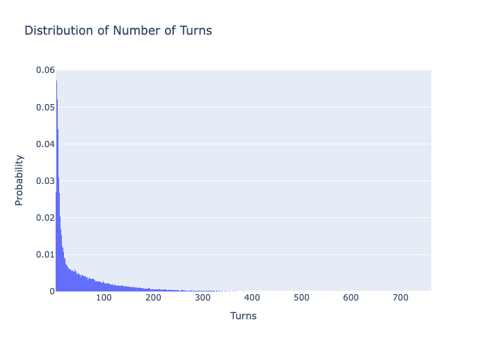
Now, lets run hundred thousand simulations (Monte Carlo method) on this board to get an estimate of the expected number of turns it takes to win and see the distribution of turns. First we will run this simulation when only one player is playing!
This distribution makes it look like a well balanced board overall, there are few unlucky ones who would have gotten eaten by big snakes multiple times (100+ turns). By eye-balling the right-skewed probability distribution, we can see most games finish in 15 to 50 turns, with a long tail of unlucky outliers..
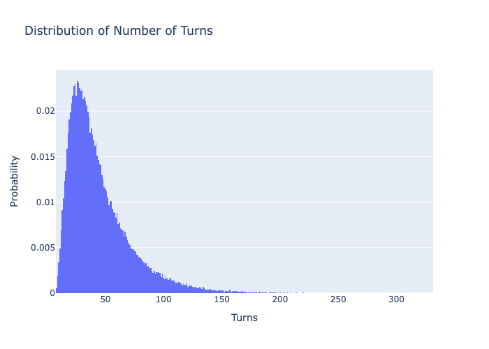
Mean: 43.82096308326311, Variance: 752.33833145564, Standard Deviation: 27.42878654726891
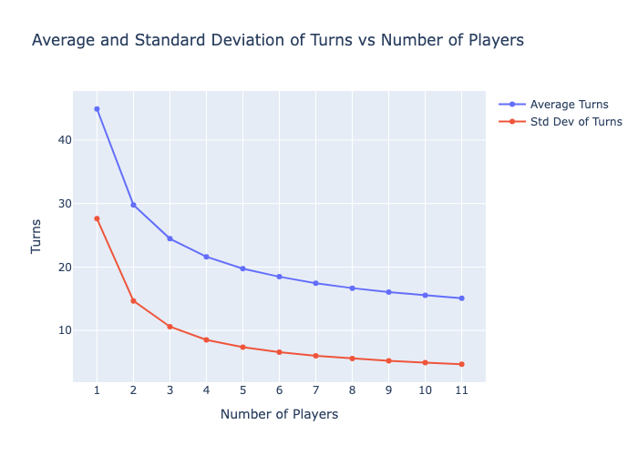
Would the game be quicker if there are more players ?
You can see below the average number of turns each player takes before someone wins. It does make intuitive sense that each player takes lesser turns, as there is higher chance of someone lucking out (falling in left side portions of probability distribution function) when there are more players. Though that doesn’t mean the game finshes quickly in the sense of time! As the total game turns itself among all players is a multiple of expected turns for each player, plus the amount of drama increases exponentially with each player :smiley:
Markov Chain Analysis
Monte Carlo simulations are great to calculate the expected number of turns, thereby helping us to understand the chances in a board. But they are also computationally expensive, especially if one wants to try out different board variations to optimize for certain factors. To our rescue are Markov Chains! Snakes and Ladders is a classic example of a Markov Chain.
- The game has a finite number of states (squares on the board).
- The probability of moving from one square to another depends only on the current square, not the history of the game.
- Say you are on square 10, and there is a ladder at square 12 -> 24, there is a snake at square 15 -> 6, the 10th row of transition matrix looks like this (0…1/6 0 0 0 0 1/6 0 1/6 1/6 0 1/6 …. 1/6 0 … ). Where the probability of each of 10 -> {6, 11, 24, 13, 14, 16} transitions have 1/6th probability and rest of the transitions have 0 probability.
By representing the board as a transition matrix and treating 100 as absorbing square, we can calculate the exact expected number of turns and the variance without running any simulations! The math behind calculation of expected number of transitions and variation in number of transitions can be found here. Let’s define a board and compare the exact Markov Chain statistics with our Monte Carlo simulation results.
Stats calculated with Monte Carlo Simulation: Mean: 44.90337, Variance: 757.3198526431, Standard Deviation: 27.519444991552792
Stats calculated with Markov Chain Process: Mean: 43.82096308326311, Variance: 752.33833145564, Standard Deviation: 27.42878654726891
More power to the law of large numbers!! The mean, variance, standard deviation calculated with Markov Chain Statistical Model are almost same as the ones we calculated from 100000 Monte Carlo Simulations.
Designing Snakes And Ladder Board Design
Now comes the interesting part.
The board we have been analyzing so far is based on what we got from the store. I’d say its a well designed board, balancing the excitement with boredom. Now, how can we design boards optimized for special cases. Say we want a board that is very chaotic, where its hard to predict how many turns it is going to take to complete the game. How about a boring board, where no matter who plays the number of turns thereby the time taken is pretty much the same.
Here we design the boards for these extreme cases, demonstrating our optimization algorithm. Before we do though, a bit on the theory:
Optimization Algorithm
We want the algorithm to figure out where to place the snakes and ladders so as to achieve the objective we are choosing for. This is a combinatorial problem, and considering the number of overall possibilities, we can’t brute force our way out of it. And here, we aren’t trying to solve for a theoretically bounded solution but a solution that we can arguable verify that it is closer to our objective.
Such optimization algorithm typically has three ingredients:
1) Loss function
The loss function we choose for is, how much the mean and standard deviation of number of turns differs from the target. So closer the mean and std to our targets, smaller the loss. weight_mean and weight_std are hyperparameters to tune for, indicating which of the component of loss function is more important.
loss = weight_mean * abs(mean - target_mean) + weight_std * abs(std - target_std)
2) Neighbour selection function
Given certain locations of snakes and the ladders, this function outputs an altered positions of these snakes and ladders, resulting in a new board. The way we alter the positions could be very wild - flipping the direction of snake/ladder, adding a new snake/ladder, swapping the positions of snake to ladder or vice versa etc. Or the alterations could be very minimal - making the snake/ladder bigger/shorter by few squares, sliding the snake/ladder but keeping length the same etc. In re-inforcement learning terminology, these moves can be categorized as exploration and exploitation respectively. Exploration moves especially at the beginnning of the game are useful to literally explore possibilities trying to get in the neighbourhood of low “energy” regions. Whereas, exploration moves are important to tune the board to get closer and closer to the objective.
My Neighbour function picks exploration move with high probability at the earlier iterations, and chooses exploitation move with high probability in final stages.
In below, _T refers to Temperature, which will talk about as part of next ingredient.
cooling_ratio = current_T / max_T

explore_pct = 0.05 + (0.55 * cooling_ratio)

explore_moves = ['add_delete', 'flip', 'swap']
exploit_moves = ['slide', 'shift', 'stretch']

if random.random() < explore_pct:
    move_type = random.choices(explore_moves, weights=[0.5, 0.3, 0.2])[0]
else:
    move_type = random.choices(exploit_moves, weights=[0.4, 0.4, 0.2])[0]
I have also put some constraints on how the board should look like, such as it should contain at least 5 snakes/ladders and at most 10, the snake/ladder shouldn’t end in same row. This is to avoid weird looking boards.
3) Iterative Loop
This is where we orchestrate the overall algorithm. We start with a random initialization of the board, and ask our Neighbour function to make a new board out of it, then we measure the loss value of the new board using the above Markov Evaluator. If the new board has lower loss, we always accept it. If the new board has higher loss than the previous version, we might still accept it with a probability that is proportional to the current temperature (math.exp(-delta_E / current_T)). The reason to accept such bad boards is to potentially escape local minima, and explore other possibilities especially at the beginning of the algorithm.
This is the same temperature that we use to derive exploitation probability in Neighbour function. Temperature can be thought of as a “risk tolerance” parameter that controls the “wildness” or randomness of the algorithm. Typically, we start with a very high temperature (max_T) and decay it in every step with a scheduled cooling ratio. So basically, at the earlier iterations of the algorithm we are very open to wild board and after some iterations we try to minimize the risk.
One note on cooling ratio is, higher this ratio and faster is the algorithm at the risk of not exploring lot of solutions.
Boring board
To design a boaring board, we set target mean as something resonable like 45 and set target standard deviation as 0
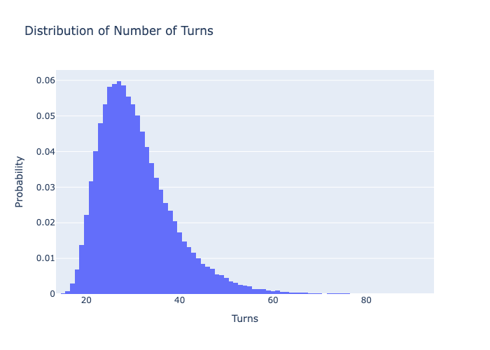
The algorithm after running ~2000 iterations produces very good, which I mean very boring board with an average of ~28 turns and a standard deviation of only ~8 turns. That means most of the the games should have 17 to 29 turns, compared to 15 to 50 turns of the original board.
Store-bought board stats: Mean: 43.82096308326311, Variance: 752.33833145564, Standard Deviation: 27.42878654726891
Boring board stats: Mean: 29.769746404989455, Variance: 64.5211715766194, Standard Deviation: 8.032507178746831
By looking at the boring board, there are definitely bare minimum snakes and ladders. Especially, the snakes are very small and they seem to be placed not to hurt you but to satisfy the constraints!
Chaotic board
Maths says that to design a chaotic or very uncertain board where we can’t really tell how long the game is going to last, we’d need to target for very high standard deviation. So we choose a reasonable mean, and a standard deviation that is higher than the mean itself.
Now, let’s try the opposite: a highly “chaotic” board. We’ll set the target mean to 45 turns again, but increase the target standard deviation to 50. This creates a highly unpredictable board where games could end extremely quickly or take forever!
Store-bought board stats: Mean: 43.82096308326311, Variance: 752.33833145564, Standard Deviation: 27.42878654726891
Chaotic board stats: Mean: 53.554156747278846, Variance: 4891.157442564327, Standard Deviation: 69.93681035452165
I really love this chaotic board! Its like either you get those very first 15, 17, 18, 19 ladders or you pretty much don’t get any help at all afterwords. Plus the snakes at 67, 68, 69, 70, 71 are like “almost” traps to increase number of turns in the game, thereby increasing the std deviation. Not sure how the algorithm came up with these placements but it is such a beautiful idea to satisfy the given loss function.
Conclusion
We have used two extreme examples to illustrate the power of stochastic optimization, and similar strategy could be use to design things for whatever value function. While this is a powerful framework that can be applied across domains and problems, designing the Loss and Neighbour functions need deep understanding of the domain. Plus in my opinion its more of an art to come up with these functions. That makes this framework even more beautiful.
Source code for simulation: https://github.com/psrikanthm/snakes-and-ladder